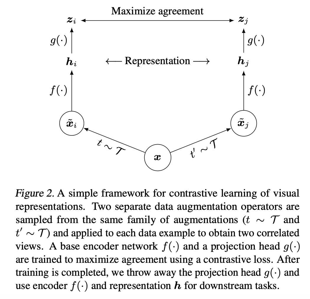
SimCLR is a simple contrastive learning framework which uses 2 augmented views of the same image and InfoNCE loss for training. Different views of the same image are considered as positive examples whereas all the other images images in a batch are considered as negatives.

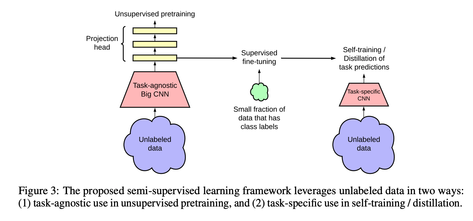
SimCLR has a follow up paper with few minor changes and improvements. Code difference between SimCLR and SimCLR V2 are minimal and there is good amount of overlap, that is why both versions are implemented here in the same module. Also, SimCLR V2 is more about the added step of knowledge distillation rather than the contrastive learning itself.
One difference in SimCLR V2 is that
MLPmodule has 3 layers instead of 2.Another difference is using a larger model for the pretraining/self supervised learning task. It is mentioned in the original paper that scaling up the model from ResNet-50 to ResNet-152 (3×+SK) gave 29% relative gain in top-1 accuracy when fine tuning with only 1% labeled data.
- Also, a few addition to data augmentation pipeline happenned, such as adding gaussian blur.
Note that self_supervised.augmentations module is highly flexible, supporting all the augmentations from the popular self supervised learning algorithms by default, allowing to pass any custom augmentations and more. It should always be adjusted based on the data and problem at hand for best performance.
Qote from SimCLR V2 paper: In our experiments, we set the width of projection head’s middle layers to that of its input, so it is also adjusted by the width multiplier. However, a wider projection head improves performance even when the base network remains narrow.
SimCLR model consists of an encoder and a projector (MLP) layer. The definition of this module is fairly simple as below.
Instead of directly using SimCLRModel by passing both an encoder and a projector, create_simclr_model function can be used by minimally passing a predefined encoder and the expected input channels.
You can use self_supervised.layers module to create an encoder. It supports all timm and fastai models available out of the box.
We define number of input channels with n_in, projector/mlp's hidden size with hidden_size, projector/mlp's final projection size with projection_size and projector/mlp's number of layers with nlayers.
encoder = create_encoder("tf_efficientnet_b0_ns", n_in=3, pretrained=False, pool_type=PoolingType.CatAvgMax)
model = create_simclr_model(encoder, hidden_size=2048, projection_size=128, nlayers=2)
out = model(torch.randn((2,3,224,224))); out.shape
The following parameters can be passed;
- aug_pipelines list of augmentation pipelines List[Pipeline] created using functions from
self_supervised.augmentationsmodule. EachPipelineshould be set tosplit_idx=0. You can simply useget_simclr_aug_pipelinesutility to get aug_pipelines. - temp temperature scaling for cross entropy loss (defaults to paper's best value)
SimCLR algorithm uses 2 views of a given image, and SimCLR callback expects a list of 2 augmentation pipelines in aug_pipelines.
You can simply use helper function get_simclr_aug_pipelines() which will allow augmentation related arguments such as size, rotate, jitter...and will return a list of 2 pipelines, which we can be passed to the callback. This function uses get_multi_aug_pipelines which then get_batch_augs. For more information you may refer to self_supervised.augmentations module.
Also, you may choose to pass your own list of aug_pipelines which needs to be List[Pipeline, Pipeline] where Pipeline(..., split_idx=0). Here, split_idx=0 forces augmentations to be applied in training mode.
aug_pipelines = get_simclr_aug_pipelines(size=28, rotate=False, jitter=False, bw=False, blur=False, stats=None, cuda=False)
aug_pipelines
DistributedSimCLR is a distributed implementation of InfoNCE Loss. It effectively increases the number of negative samples to all available samples across all GPUs during loss calculation. For example, if you use batch size of 16 per GPU and 8 GPUs, then the loss will be calculated using a similarity matrix with size of 16x8 x 16x8 = 1024x1024. In literature/experiments it's mentioned that more negatives help training.
Following callback should be used together with DistributedDataParallel and inside a python script which will be executed in launch mode, such as:
python -m fastai.launch script.py --FOLD 4 --size 640 --bs 12 --epochs 10 --lr 1e-3 --arch_name tf_efficientnet_b7_ns
For more details about distributed operations like all gather, see https://pytorch.org/tutorials/intermediate/dist_tuto.html.
Training Tip: You can maximize your effective batchsize by using gradient checkpointing (see self_supervised.layers module), fp16 (Learner.to_fp16() in fastai) and distributed callback. Don't worry if you don't have access to multiple GPUs, usually just using gradient checkpointing and fp16 is enough to increase your batch size to 256 and beyond. Which is enough to train highly competitive models.
path = untar_data(URLs.MNIST_TINY)
items = get_image_files(path)
tds = Datasets(items, [PILImageBW.create, [parent_label, Categorize()]], splits=GrandparentSplitter()(items))
dls = tds.dataloaders(bs=5, after_item=[ToTensor(), IntToFloatTensor()], device='cpu')
fastai_encoder = create_encoder('xresnet18', n_in=1, pretrained=False)
model = create_simclr_model(fastai_encoder, hidden_size=2048, projection_size=128)
aug_pipelines = get_simclr_aug_pipelines(size=28, rotate=False, jitter=False, bw=False, blur=False, stats=None, cuda=False)
learn = Learner(dls, model, cbs=[SimCLR(aug_pipelines, temp=0.07, print_augs=True),ShortEpochCallback(0.001)])
Also, with show_one() method you can inspect data augmentations as a sanity check. You can use existing augmentation functions from augmentations module.
b = dls.one_batch()
learn._split(b)
learn('before_batch')
axes = learn.sim_clr.show(n=5)
learn.fit(1)
learn.recorder.losses
